Introduction:
One of the main challenges in quantum computing is the noise in current devices. In this task, you will create a simple noise generator and assess its effect. You can use any framework you like (Qiskit, Cirq, etc..)
Noise Model
A standard way to represent the noise in a quantum circuit is through Pauli operators (x, y, z). Build a function with input , and QuantumCircuit where:
→ Probability of having a random Pauli operator acting on the qubit after a one-qubit gate → Probability of having a random Pauli operator acting on the qubit after a two-qubit gate QuantumCircuit → Quantum circuit where the noise will be added
The output should be the Quantum Circuit with Noise
Gate Basis
Quantum computers can implement only a set of gates that, with transformations, can represent any other possible gate. This set of gates is called the Gate Basis of the QPU. Build a function that transforms a general Quantum Circuit to the following gate basis: {CX,ID,RZ,SX,X}
Adding two numbers with a quantum computer
Build a function (quantum_sum) to add two numbers using the Draper adder algorithm. You will need the Quantum Fourier Transform (QFT). Many libraries offer a function to use it. For this task, you will need to build QFT from scratch.
Effects of noise on quantum addition
Now, we can combine all the functions. Transform the circuit used in the quantum_sum to the gate basis and add noise. Use different levels of noise and analyze the results.
How does the noise affect the results? Is there a way to decrease the effect of noise? How does the number of gates used affect the results?
References:
[3] Quantum arithmetic with the Quantum Fourier Transform https://arxiv.org/pdf/1411.5949.pdf
import pennylane as qml
import pennylane.numpy as np
from pennylane.pauli import PauliWord, PauliSentence
from pennylane.drawer import tape_mpl
import matplotlib as plt
import pandas as pd

import warnings
warnings.filterwarnings("ignore")
Step one: Add noise
A standard way to represent the noise in a quantum circuit is through Pauli operators ($\sigma_x, \sigma_y, \sigma_z$). Build a function with input $\alpha$, $\beta$ and QuantumCircuit where:
$\alpha$ → Probability of having a random Pauli operator acting on the qubit after a one-qubit gate
$\beta$ → Probability of having a random Pauli operator acting on the qubit after a two-qubit gate
QuantumCircuit → Quantum circuit where the noise will be added
The output should be the Quantum Circuit with Noise
There is a module qml.add_noise in pennylane to simulate noise. But I preferred to write the code from scratch:
def noisy_QC(alpha, beta, QC):

    # Extract the information about the QC:
    t = QC.tape
    ops  = t.operations
    obs  = t.observables
    mes  = t.measurements


    with qml.tape.QuantumTape() as tape_new:
        for g in ops:
            qml.apply(g)
            if len(g.wires) == 1: #1-qbit gate noise
                w = g.wires[0]
                paulis = ['X','Y','Z']
                choice = np.random.randint(2)
                noise =  PauliSentence({PauliWord({0:'I'}): np.sqrt((1-alpha)),
                                        PauliWord({0:paulis[choice]}): np.sqrt(alpha) })
                U_noise = noise.to_mat()
                qml.QubitUnitary(U_noise,wires = w, id = 'Alpha')


            elif len(g.wires) == 2: #2-qbit gate noise
                w = g.wires[1]
                paulis = ['X','Y','Z']
                choice = np.random.randint(2)
                noise =  PauliSentence({PauliWord({0:'I'}): np.sqrt(1-beta),
                                        PauliWord({0:paulis[choice]}): np.sqrt(beta) })
                U_noise = noise.to_mat()
                qml.QubitUnitary(U_noise,wires = w, id = 'Beta')

        [qml.apply(mes[i]) for i in range(len(mes))]

    return tape_new
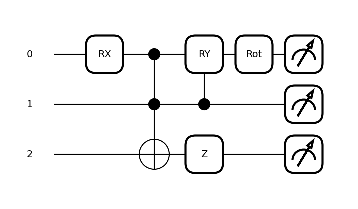
Consdier the follwing example circuite and let’s check how adding noisy gates works:
dev_test = qml.device('default.qubit', wires=4)
@qml.qnode(dev_test)

def circuit(x, y):
    qml.RX(x[0], wires=0)
    qml.Toffoli(wires=(0, 1, 2))
    qml.CRY(x[0], wires=(1, 0))
    qml.Rot(x[2], x[3], y, wires=0)
    qml.PauliZ(2)
    return qml.state()

x = np.array([0.05, 0.1, 0.8, 0.3], requires_grad=True)
y = np.array(0.4, requires_grad=False)
x = np.array([0.05, 0.1, 0.8, 0.3], requires_grad=True)
y = np.array(0.4, requires_grad=False)

print(qml.draw_mpl(circuit)(x, y))
(<Figure size 700x400 with 1 Axes>, <Axes: >)
x = np.array([0.05, 0.1, 0.8, 0.3], requires_grad=True)
y = np.array(0.4, requires_grad=False)
test = circuit(x, y)
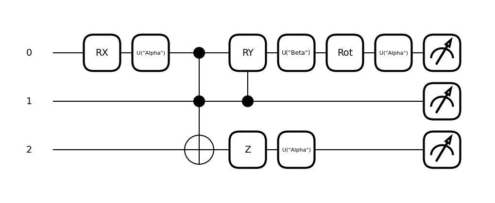
tape_noisy = noisy_QC(alpha = 0.7, beta = 0.12, QC = circuit)
fig, ax = tape_mpl(tape_noisy)
fig.show()
/var/folders/94/tm2kp09x4vs6xb2y11f7qjjm0000gn/T/ipykernel_48329/115943239.py:10: UserWarning: FigureCanvasAgg is non-interactive, and thus cannot be shown
  fig.show()
Step Two: Gate decomposition and Arrpoximation
Gate Basis
Quantum computers can implement only a set of gates that, with transformations, can represent any other possible gate. This set of gates is called the Gate Basis of the QPU. Build a function that transforms a general Quantum Circuit to the following gate basis: {CX,ID,RZ,SX,X}
I used the buit_in module for Solovay-Kitaev decomposition. It turns out there is a bug in pennylanes module. It is said that the code first decomposes the the 1-qbit gates to {H, S, SX, X, T etc} and then use Solovay-Kitaev to find an apporximation for RZ gates. However the module, for single qbits part, uses another module that doesn’t work with “SX” as basis. Since writing the code from scratch could take too long, I decided to use {S, H, X} basis for single qbit gates. In principle, one can replace the H-gates with SX and S. And S gates with RZ and a phase. So it wouldn’t be hard to modify this …
def decomposed_circuit(circ):

    basis = ('I','S','H','X')

    return qml.transforms.clifford_t_decomposition(circ,epsilon=0.01, method = 'sk', basis_set = basis )
Step Three: Quantum Adder
Adding two numbers with a quantum computer
I’ll build a function (quantum_sum) to add two numbers using the Draper adder algorithm. You will need the Quantum Fourier Transform (QFT). Many libraries offer a function to use it. For this task, I will build QFT from scratch.
In the following code, I first tranfored numbers into binaries, then I used PaulisWord to define the initial states.
In the next code, I will use QuantumStateVector.
def quantum_sum( num_x, num_y, num_qbits = 10): #num_qubits := # of qubits
                                                #num_x and num_y the number to be added.
                                                #only num_y will be transformed into binary series


    phi = 2*np.pi/(2**num_qbits)

    bin_y = bin(num_y)[2:]
    bin_y = '0'*(num_qbits - len(bin_y)) + bin_y
    state_y = np.array( [ int(bin_y[i]) for i in range(len(bin_y)) ] ) #This state will be fed into QFT_circuit

    dev = qml.device('default.qubit',wires=num_qbits)
    @qml.qnode(dev)


    def QFT_circuit (input_state, num_qbits = num_qbits): #Take the initial state as an array-like of binaries
                                                                       #This Function is not exactly as QFT
                                                                       #The final state have to be reordered.
                                                                       #Reordering is done in another function

        #Preparing the initial state:

        paulidict = {0:'I', 1: 'X'}
        initial_state = PauliWord({i: paulidict[ int(input_state[i]) ] for i in range(num_qbits) })
        if all(input_state == 0): qml.Identity
        else:
            U_I = initial_state.to_mat()
            qml.QubitUnitary(U_I ,wires = initial_state.wires) # I used this gate to deine an initial state
                                                               # correspoinding to binary numbers.


         #The QFT operator:

        qml.Hadamard(wires = 0)
        for w in range(1,num_qbits):
            phi_w = (phi)*(input_state[w] * 2**(num_qbits - w -1))

            for crp in range(w):
                U = np.array([[np.exp(1j*phi_w * (2**(crp))), 0  ],
                             [0, np.exp(1j*phi_w * (2**(crp)))   ]])
                qml.ControlledQubitUnitary(U, control_wires = crp , wires = w)

            qml.Hadamard(w)

        return qml.state()

    def qft(state_vect, Inverse = False): #When Inverse is true, it computes the Inverse QFT.
        st = QFT_circuit(state_vect, num_qbits)

        def rev_bin(b): # This function is for reordering the output only.
            bin_b =  bin(b)[2:]
            bin_b = '0'*(num_qbits - len(bin_b)) + bin_b
            binary = bin_b[::-1]
            return int(binary, 2)

        qft0 = np.zeros(2**num_qbits, dtype=complex)
        for i in range(2**num_qbits):
            if Inverse:
                qft0[rev_bin(i)] = np.conj(st[i])
            else:
                qft0[rev_bin(i)] = st[i]

        return qft0


    state_qft_y = qft(state_y, Inverse = False)

    # The follwing state, ctrl_Z, will be given to the inverse_QFT:

    ctrl_Z = np.array([state_qft_y[i] *  np.exp(1j*phi * (i * num_x)) for i in range(2**num_qbits) ] )

    final_state = np.zeros(2**num_qbits)

    for num_z in range(2**num_qbits):

        bin_z = bin(num_z)[2:]
        bin_z = '0'*(num_qbits - len(bin_z)) + bin_z
        state_z = np.array( [ int(bin_z[i]) for i in range(len(bin_z)) ] )

        state_qftI_z = qft(state_z, Inverse = True)

        final_state = final_state + ctrl_Z[num_z] * state_qftI_z


    return np.argmax(final_state * final_state.conj())
# 1+15 mod 16
quantum_sum( num_x=15, num_y=1, num_qbits = 4)
0
# 1+10 mod 16
quantum_sum( num_x=10, num_y=1, num_qbits = 4)
11
In the table below, you see the result of quantum addition mod 16 ( 4 qubits)
df = pd.DataFrame(columns = [i for i in range(16)], index = [i for i in range(16)])
for indx in range(df.shape[0]):
    for cn in range(df.shape[1]):
        df.iloc[indx,cn] = quantum_sum( num_x=indx, num_y=cn, num_qbits = 4)
df
| 0 | 1 | 2 | 3 | 4 | 5 | 6 | 7 | 8 | 9 | 10 | 11 | 12 | 13 | 14 | 15 | |
|---|---|---|---|---|---|---|---|---|---|---|---|---|---|---|---|---|
| 0 | 0 | 1 | 2 | 3 | 4 | 5 | 6 | 7 | 8 | 9 | 10 | 11 | 12 | 13 | 14 | 15 |
| 1 | 1 | 2 | 3 | 4 | 5 | 6 | 7 | 8 | 9 | 10 | 11 | 12 | 13 | 14 | 15 | 0 |
| 2 | 2 | 3 | 4 | 5 | 6 | 7 | 8 | 9 | 10 | 11 | 12 | 13 | 14 | 15 | 0 | 1 |
| 3 | 3 | 4 | 5 | 6 | 7 | 8 | 9 | 10 | 11 | 12 | 13 | 14 | 15 | 0 | 1 | 2 |
| 4 | 4 | 5 | 6 | 7 | 8 | 9 | 10 | 11 | 12 | 13 | 14 | 15 | 0 | 1 | 2 | 3 |
| 5 | 5 | 6 | 7 | 8 | 9 | 10 | 11 | 12 | 13 | 14 | 15 | 0 | 1 | 2 | 3 | 4 |
| 6 | 6 | 7 | 8 | 9 | 10 | 11 | 12 | 13 | 14 | 15 | 0 | 1 | 2 | 3 | 4 | 5 |
| 7 | 7 | 8 | 9 | 10 | 11 | 12 | 13 | 14 | 15 | 0 | 1 | 2 | 3 | 4 | 5 | 6 |
| 8 | 8 | 9 | 10 | 11 | 12 | 13 | 14 | 15 | 0 | 1 | 2 | 3 | 4 | 5 | 6 | 7 |
| 9 | 9 | 10 | 11 | 12 | 13 | 14 | 15 | 0 | 1 | 2 | 3 | 4 | 5 | 6 | 7 | 8 |
| 10 | 10 | 11 | 12 | 13 | 14 | 15 | 0 | 1 | 2 | 3 | 4 | 5 | 6 | 7 | 8 | 9 |
| 11 | 11 | 12 | 13 | 14 | 15 | 0 | 1 | 2 | 3 | 4 | 5 | 6 | 7 | 8 | 9 | 10 |
| 12 | 12 | 13 | 14 | 15 | 0 | 1 | 2 | 3 | 4 | 5 | 6 | 7 | 8 | 9 | 10 | 11 |
| 13 | 13 | 14 | 15 | 0 | 1 | 2 | 3 | 4 | 5 | 6 | 7 | 8 | 9 | 10 | 11 | 12 |
| 14 | 14 | 15 | 0 | 1 | 2 | 3 | 4 | 5 | 6 | 7 | 8 | 9 | 10 | 11 | 12 | 13 |
| 15 | 15 | 0 | 1 | 2 | 3 | 4 | 5 | 6 | 7 | 8 | 9 | 10 | 11 | 12 | 13 | 14 |
Step Four: Noise effect
Now, we can combine all the functions. Transform the circuit used in the quantum_sum to the gate basis and add noise. Use different levels of noise and analyze the results.
How does the noise affect the results?
Is there a way to decrease the effect of noise?
How does the number of gates used affect the results?
def noisy_adder(num_x, num_y, num_qbits, alpha, beta):

    phi = 2*np.pi/(2**num_qbits)

    bin_y = bin(num_y)[2:]
    bin_y = '0'*(num_qbits - len(bin_y)) + bin_y
    state_y = np.array( [ int(bin_y[i]) for i in range(len(bin_y)) ] ) #This state will be fed into QFT_circuit

    dev = qml.device('default.qubit',wires=num_qbits)
    @qml.qnode(dev)


    def QFT_circuit (input_state, num_qbits = num_qbits): #Take the initial state as an array-like of binaries
                                                                       #This Function is not exactly as QFT
                                                                       #The final state have to be reordered.
                                                                       #Reordering is done in another function

        #Preparing the initial state:

        l = len(input_state)
        initial_state = np.zeros(2**l, dtype = complex)
        ind = 0
        state_y
        for i in range(l):
            ind += input_state[i]*(2** (l - i -1 ) )

        initial_state[int(ind)] = 1.0 + 0.0*1j
        qml.QubitStateVector(initial_state, wires=[i for i in range(num_qbits)])


         #The QFT operator:

        qml.Hadamard(wires = 0)
        for w in range(1,num_qbits):
            phi_w = (phi)*(input_state[w] * 2**(num_qbits - w -1))

            for crp in range(w):
                U = np.array([[np.exp(1j*phi_w * (2**(crp))), 0  ],
                             [0, np.exp(1j*phi_w * (2**(crp)))   ]])
                qml.ControlledQubitUnitary(U, control_wires = crp , wires = w)

            qml.Hadamard(w)

        return qml.state()

    ST_QFT = decomposed_circuit(QFT_circuit)


    def qft(state_vect, Inverse = False): #When Inverse is true, it computes the Inverse QFT.
        test = ST_QFT(state_vect)
        noisy_QFT = noisy_QC(alpha = alpha, beta = beta , QC = ST_QFT)

        st = qml.execute([noisy_QFT],dev)[0]

        def rev_bin(b): # This function is for reordering the output only.
            bin_b =  bin(b)[2:]
            bin_b = '0'*(num_qbits - len(bin_b)) + bin_b
            binary = bin_b[::-1]
            return int(binary, 2)

        qft0 = np.zeros(2**num_qbits, dtype=complex)
        for i in range(2**num_qbits):
            if Inverse:
                qft0[rev_bin(i)] = np.conj(st[i])
            else:
                qft0[rev_bin(i)] = st[i]

        return qft0


    state_qft_y = qft(state_y, Inverse = False)

    # The follwing state, ctrl_Z, will be given to the inverse_QFT:

    ctrl_Z = np.array([state_qft_y[i] *  np.exp(1j*phi * (i * num_x)) for i in range(2**num_qbits) ] )

    final_state = np.zeros(2**num_qbits)

    for num_z in range(2**num_qbits):

        bin_z = bin(num_z)[2:]
        bin_z = '0'*(num_qbits - len(bin_z)) + bin_z
        state_z = np.array( [ int(bin_z[i]) for i in range(len(bin_z)) ] )

        state_qftI_z = qft(state_z, Inverse = True)

        final_state = final_state + ctrl_Z[num_z] * state_qftI_z

    res = np.argmax(final_state * final_state.conj())

    tape = ST_QFT.tape
    num_gates = len(tape.operations)
    return res, num_gates
# 2+4 mod 8 with noise
noisy_adder(num_x=2, num_y=4, num_qbits=3, alpha=0.001, beta=0.001)
(6, 7)
alpha_effect = []
for i in range(10):
    res = noisy_adder(num_x=2, num_y=4, num_qbits=3, alpha=0.00 + 0.05*i, beta=0.001)[0]
    alpha_effect.append(res)
alpha_effect
[6, 6, 6, 6, 6, 6, 6, 7, 3, 7]
beta_effect = []
for i in range(10):
    res = noisy_adder(num_x=2, num_y=4, num_qbits=3, alpha=0.001, beta=0.00+0.05*i)
    beta_effect.append(res)
beta_effect
[(6, 7),
 (6, 7),
 (6, 7),
 (0, 7),
 (0, 7),
 (0, 7),
 (2, 7),
 (1, 7),
 (1, 7),
 (4, 7)]
beta_effect_r = [beta_effect[i][0] for i in range(10)]
import matplotlib.pyplot as plt

#plt.figure(figsize = (17,5))

#plt.subplot(131)
plt.plot(range(10), alpha_effect, label = 'Alpha noise effect')
plt.plot(range(10),beta_effect_r, label = 'Beta noise effect')
plt.legend()
plt.xlabel('Noise probability [0.05 steps]')
plt.ylabel('Result')
plt.title('The effect of noise on Quantum_sum(2+4) accuracy (3 Qbits)')

plt.show()
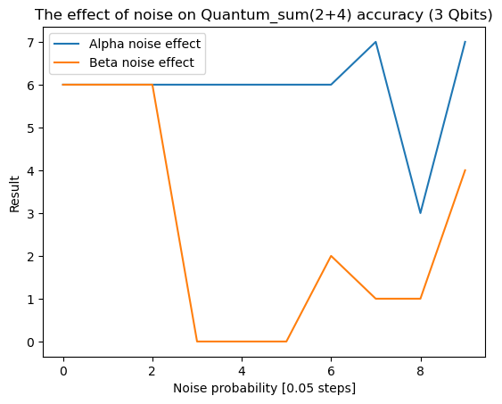
The effect of noises on the accuracy of the quantum circuit is shown on this graph
The follwoign part is too slow on my computer. I had to interrupt the kernel after a while. But it generated enough data:
Please check end of the file.
import time

gate_effect = []
gate_time = []
for i in range(4):
    start = time.time()
    res = noisy_adder(num_x=2, num_y=1, num_qbits=2+i, alpha=0.001, beta=0.001)
    end = time.time()
    gate_time.append(end-start)
    beta_effect.append(res)
gate_effect
gate_time
[0.284862756729126, 57.56048011779785, 213.88656377792358, 1111.6123750209808]
gate_effect = beta_effect[-4:]
gate_effect
[(3, 4), (3, 7), (3, 11), (3, 16)]
plt.figure(figsize = (12,6))


plt.subplot(121)
plt.plot( [gate_effect[i][1] for i in range(4)], gate_time )
plt.xlabel('Number of Gates')
plt.ylabel('Time(s)')
plt.title('Effect of Gate number in timing')

plt.subplot(122)
plt.plot(range(2,6), [gate_effect[i][1] for i in range(4)] )
plt.ylabel('Number of Gates')
plt.xlabel('Number of Qbits')

plt.show()
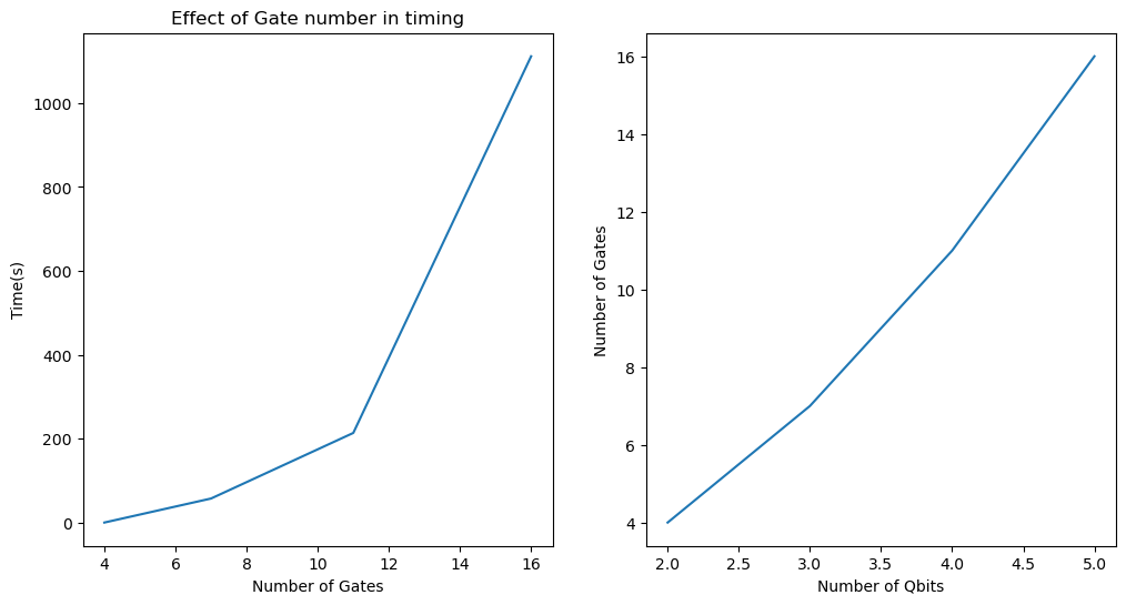
These graphs shows time needed to complete the computaion grows exponentially in term of number of gates.
The growth in number of gates is almost linear relative to the number of Qbits
The noise caused by Z corresponds to phase flip and the noise caused by X is the bir flip error. Y is combination of both.
It is possible generally to use error correction codes to reduce the effect of these errors